Reports with RMarkdown

Overview

Teaching: 80 min
Exercises: 35 min

Questions

Why should you use RMarkdown to produce your manuscripts?

What are the advantages of using RMarkdown vs Word or LaTeX

Objectives

Become familiar with RMarkdown document structure

Use basic formating syntax

Learn to weave prose and code together

Acknowledgments

This lesson has been heavily influence by the Tobin Magle’s presentation created for the UW-Madison’s Library Research Guides entitled “Creating reproducible Research using R Markdown.”

Agenda

Why should you write your reports using RMarkdown?
What is literate programming? Why is it useful?
Scenario: Using R Markdown to
- Format text
- Embed code
- Run Analyses
- Create Tables
- Create Plots
Create your own document
Ideas to organize your document
Summary
Where to find help

Why you should write your reports using RMarkdown?

Rather than telling you why, I’m going to show you what the usual workflow for manuscript production in my field looks like. Then I’m going to show you what it looks like now that I have switched to writing exclusively in RMarkdown.

collect data (interviews, recordings, corpora)
code it into some type of data (tokens, measurements, categories)
enter that into some computer software for analysis and visualizations
write the prose in word processor
copy and paste the results from the analysis software
import plots into the word processor
changes in the data results into repeating steps 1-6

Sounds familiar? Can we do better?

Anatomy of an RMarkdown document

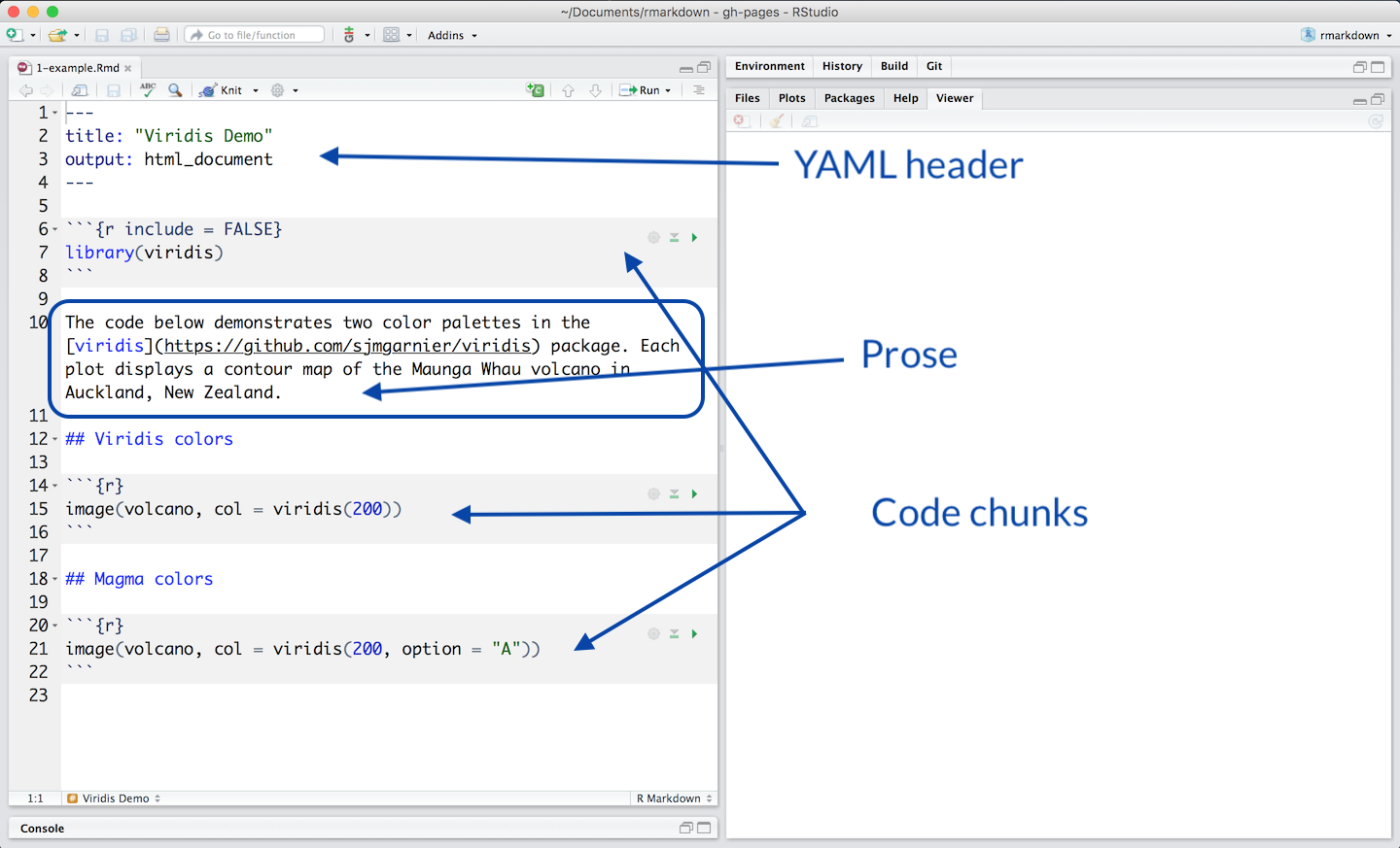
A typical RMarkdown document has three distinct parts:

1 - an (optional) YAML header surrounded by ---.
2 - your prose (optionally) formatted using Markdown syntax. It also can include inline code.
3 - Code chunks containing your R script surrounded by 3 backticks.

plot of chunk unnamed-chunk-2

Literate programming

Human readable text + machine readable code = reproducible document

Programs as work of literature

Idea by Donald Knuth, Stanford University.
A paradigm shift:
- from telling a computer what to do
- to telling a human what you want the computer to do

Tailor reports to an audience
Repeatable. Ensures reproducibility
Works well with version control
Works well with languages used in research.

R, RStudio and RMarkdown

Weave your prose and code into one cohesive story
- R
- Python
- Stata
- SAS
- LaTeX
Produce document in many formats
Reproducible

Scenario

SAFI (Studying African Farmer-Led Irrigation) is a study looking at farming and irrigation methods in Tanzania and Mozambique. The survey data was collected through interviews conducted between November 2016 and June 2017. For this lesson, we will be using a subset of the available data. For information about the full teaching dataset used in other lessons in this workshop, see the dataset description.

Install the packages you’ll need

library(markdown)
library(knitr)
library(tidyverse)
library(gt)

Play with your document

Click knit

Get the data

interviews_plotting <- read_csv(url("https://go.wisc.edu/5id64b"))

head(interviews_plotting)

# A tibble: 6 x 45
  key_ID village interview_date      no_membrs years_liv respondent_wall_… rooms
   <dbl> <chr>   <dttm>                  <dbl>     <dbl> <chr>             <dbl>
1      1 God     2016-11-17 00:00:00         3         4 muddaub               1
2      1 God     2016-11-17 00:00:00         7         9 muddaub               1
3      3 God     2016-11-17 00:00:00        10        15 burntbricks           1
4      4 God     2016-11-17 00:00:00         7         6 burntbricks           1
5      5 God     2016-11-17 00:00:00         7        40 burntbricks           1
6      6 God     2016-11-17 00:00:00         3         3 muddaub               1
# … with 38 more variables: memb_assoc <chr>, affect_conflicts <chr>,
#   liv_count <dbl>, no_meals <dbl>, instanceID <chr>, bicycle <lgl>,
#   television <lgl>, solar_panel <lgl>, table <lgl>, cow_cart <lgl>,
#   radio <lgl>, cow_plough <lgl>, solar_torch <lgl>, mobile_phone <lgl>,
#   motorcyle <lgl>, NULL <lgl>, fridge <lgl>, electricity <lgl>,
#   sofa_set <lgl>, lorry <lgl>, sterio <lgl>, computer <lgl>, car <lgl>,
#   Jan <lgl>, Sept <lgl>, Oct <lgl>, Nov <lgl>, Dec <lgl>, Feb <lgl>,
#   Mar <lgl>, Aug <lgl>, June <lgl>, July <lgl>, Apr <lgl>, May <lgl>,
#   none <lgl>, number_months_lack_food <dbl>, number_items <dbl>

Add some prose

The SAFI dataset contains data related to households and agriculture in Tanzania and Mozambique. The survey covers things like:

household features
agricultural practices
assets
details about the household members

Play with your document!!!

Click knit

Weave some code into it to create a narrative

Let’s imagine we want write a paragraph about the population per village. Which village is the most populated? Is it Chirodzo, God, or Ruaca?

Create a table

interviews_plotting %>% select(village, no_membrs) %>% 
  group_by(village) %>%
  summarize(population = sum(no_membrs))  %>%
  gt() %>%
  tab_header(title = md("**Studying African Farmer-Led Irrigation**"),
            subtitle = md("Population _per village_"))

Studying African Farmer-Led Irrigation
Population per village
village	population
Chirodzo	276
God	295
Ruaca	371

Version A: prose with results manually added
Of the three villages surveyed, Ruaca is the most populated with 371 people. The second-most populated village is God with 295 people. The least populated village in the sample is Chirodzo with 276.

Note

It would be ideal that the prose be responsive to the data we just produced! We can incorporate that into our document with inline code!

Version B: prose with results via inline code
First let’s store our results in an object, then let’s access the object to get the results we want.

pop_results <- interviews_plotting %>% 
  select(village,no_membrs) %>% 
  group_by(village) %>%
  summarize(population = sum(no_membrs)) 

Of the three villages surveyed, Ruaca is the most populated with 371 people.

Note

The name of the village and the population total you see in the previous sentence weren’t typed. They were extracted from the data we created using inline code. With inline code you can weave your prose with results that are responsible to changes in your data.

To get the name of the village with the most people, this code is needed `r pop_results$village[3]`. To get the actual number of inhabitants, this code is needed `r pop_results$population[3]`.

Add your own inline code

Challenge. Modify the rest of the paragraph so that the rest of the villages and their population appear in the text. Remember that the data you need the R object is contained in the object pop_result.

Solution

Of the three villages surveyed, Ruaca is the most populated with 371 people. The second-most populated village is God with 295 people. The least populated village in the sample Chirodzo with 276.

Create a plot

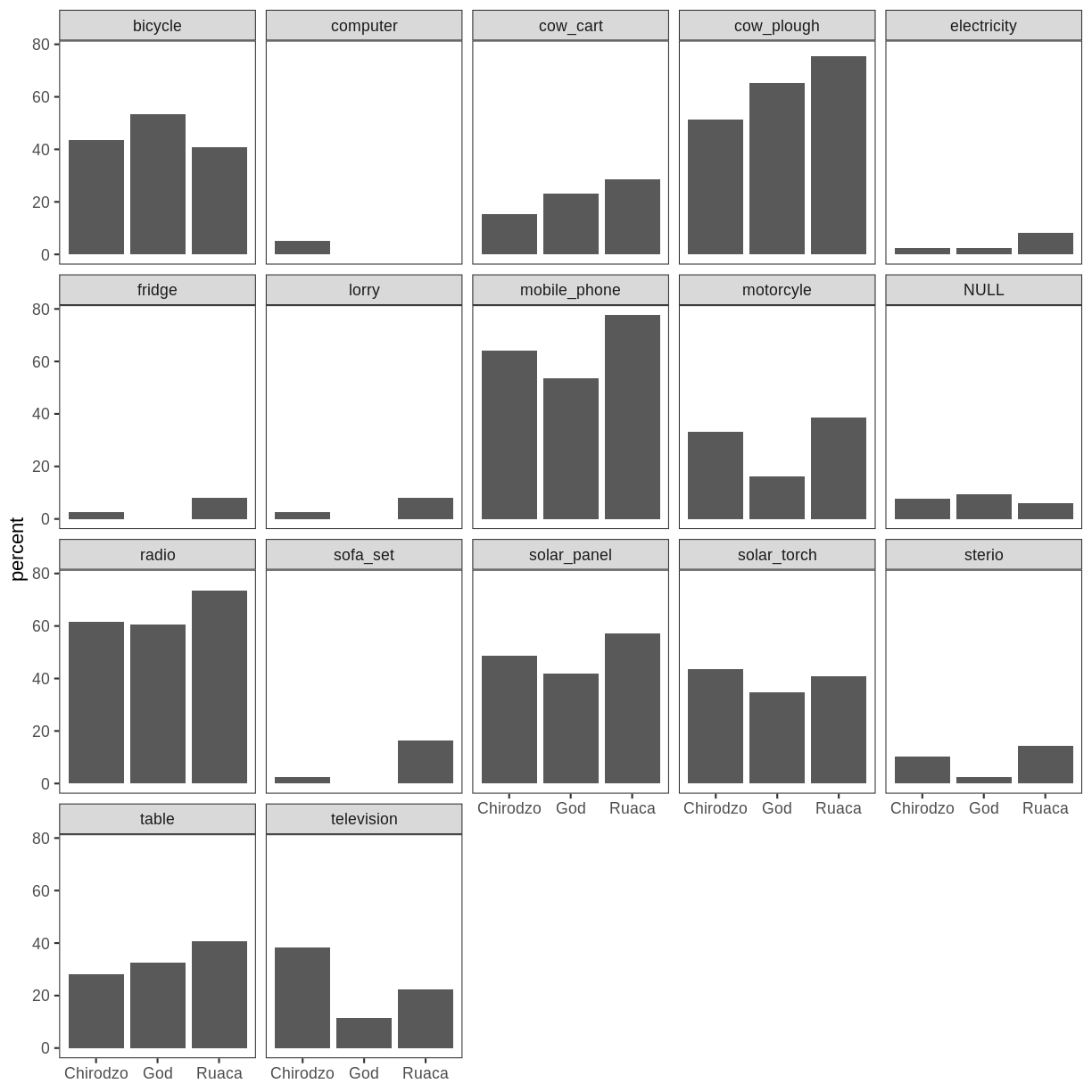
Imagine now that we want to get an idea of we want to get an idea of the type and number of items per house hold across all three villages. We can use what we learned in the ggplot lesson to create such a plot.

interviews_plotting %>% 
    group_by(village) %>%
    summarize(across(bicycle:computer, ~ sum(.x) / n() * 100)) %>% 
    pivot_longer(bicycle:computer, names_to = "items", values_to = "percent") %>% 
    ggplot(aes(x = village, y = percent)) +
    geom_bar(stat = "identity", position = "dodge") +
    facet_wrap(~ items) +
    theme_bw() +
    theme(panel.grid = element_blank(), axis.title.x = element_blank())

plot of chunk unnamed-chunk-7

Add some color

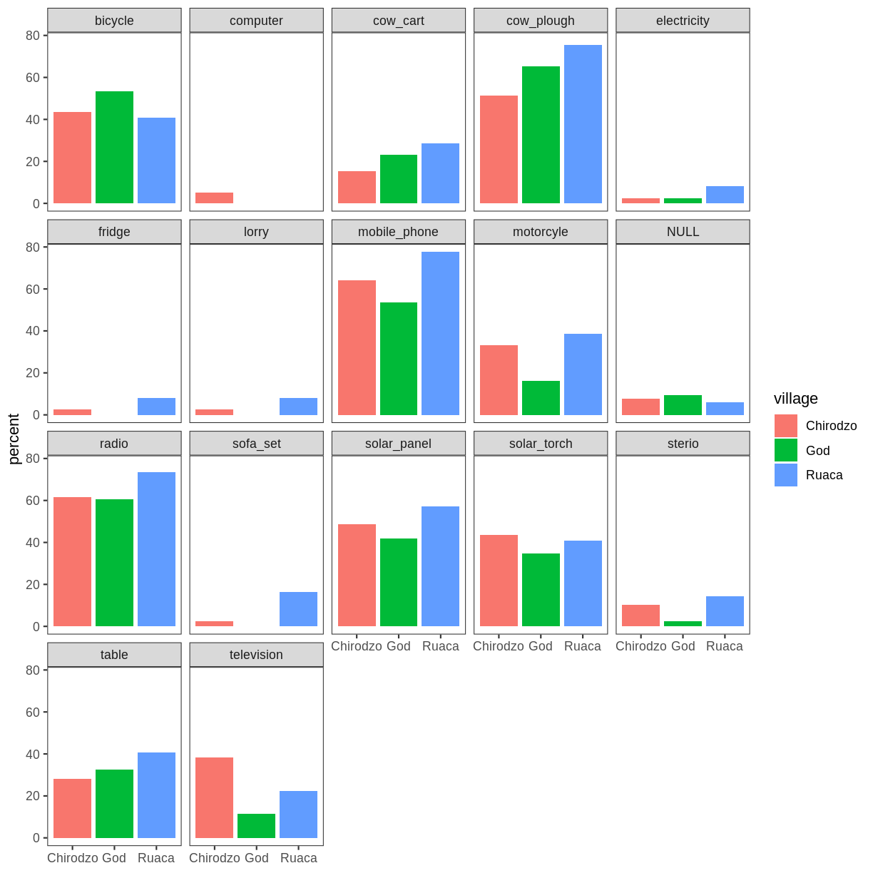
Challenge. Modify the code above so that the new barplots are color to reflect each village.

Solution

interviews_plotting %>% 
    group_by(village) %>%
    summarize(across(bicycle:computer, ~ sum(.x) / n() * 100)) %>% 
    pivot_longer(bicycle:computer, names_to = "items", values_to = "percent") %>% 
    ggplot(aes(x = village, y = percent, fill = village)) +
    geom_bar(stat = "identity", position = "dodge") +
    facet_wrap(~ items) +
    theme_bw() +
    theme(panel.grid = element_blank(), axis.title.x = element_blank())

plot of chunk unnamed-chunk-8

What’s happening behind the scenes?

plot of chunk set-a

Ideas to organize your reproducible document

Outline first, add code later
Use markdown syntax to structure and format your document # headings ** boldfacing
Check the cheatsheet

Summary

Literate programming makes reproducible research more machine readable
R markdown documents facilitate literate programming in RStudio
R markdown has 3 sections
- Header: determines output and adds parameters
- Markdown Text: it can be lightly formatted and can include inline code too!
- Code chunks: can be customized to mute code or output

Need help?

Key Points

RMarkdown document change dynamically in response to changes in the data

RMarkdown lets you instantiate literally programming easily

previous episode

R for Social Scientists

lesson home

Reports with RMarkdown

Overview

Acknowledgments

Agenda

Why you should write your reports using RMarkdown?

Anatomy of an RMarkdown document

Literate programming

Programs as work of literature

Literal Programming in Research

R, RStudio and RMarkdown

Scenario

Install the packages you’ll need

Get the data

Add some prose

Weave some code into it to create a narrative

Create a table

Note

Note

Add your own inline code

Solution

Create a plot

Add some color

Solution

What’s happening behind the scenes?

Ideas to organize your reproducible document

Summary

Need help?

Key Points

previous episode

lesson home